Agentic AI AI

构建用于语义代码搜索的 RAG 管道：开发者日记与实战笔记

第 1 部分：解析、分块与向量化

不久前，我们着手构建我们所能打造的最佳语义代码搜索平台：一个 RAG 管道，让 LLM Agent 能够从真实代码仓库中获得精确、可引用的证据，而不是依赖 grep 碰巧搜出来的内容。最终的解决方案是 Air Context。我们让它成功运行、投入生产，也在这个过程中积累了不少惨痛教训。在这一系列文章中，我们将分享那些我们希望在第一天就有人告诉我们的经验。

---

编码 Agent 无疑是本十年软件开发领域最大的技术飞跃。Agent 与前沿模型正证明，即使面对看似难以逾越的代码复杂性，它们也有能力产出表面上可靠的代码。

然而，随着越来越多的开发流程由 Agent 驱动，Agent 的效率以及其生成代码的质量变得愈发重要。问题并不完全在于 Agent 能否完成任务——只要给予足够时间和 token 资源，它当然能够完成——而在于它需要耗费多少时间、精力和引导，才能产出达到生产级标准的结果。尤其对于大规模代码库，Agent 会花费大量时间搜索与其正在开发的功能相关的代码片段，并将这些内容纳入上下文。

为什么语义搜索很重要

在尝试定位正确的代码片段时，Agent 会借助关键词搜索和 grep 等传统代码搜索工具。不过，这些工具的局限在于：它们要求 Agent 预先知道要搜索的准确文本。例如，一个需要找到会话 token 在何处刷新的 Agent，不能指望代码中恰好贴心地包含“refresh”这个词。要对抽象领域进行推理，Agent 需要能够按代码的含义进行搜索，这也就是语义搜索。检索增强生成（RAG）正是在此发挥作用。如果我们能够以捕获源代码语义的方式对它建立索引，再让 Agent 按需通过自由文本搜索检索相关片段，我们就构建了一个能够发挥 Agent 优势的接口。

从原型到生产

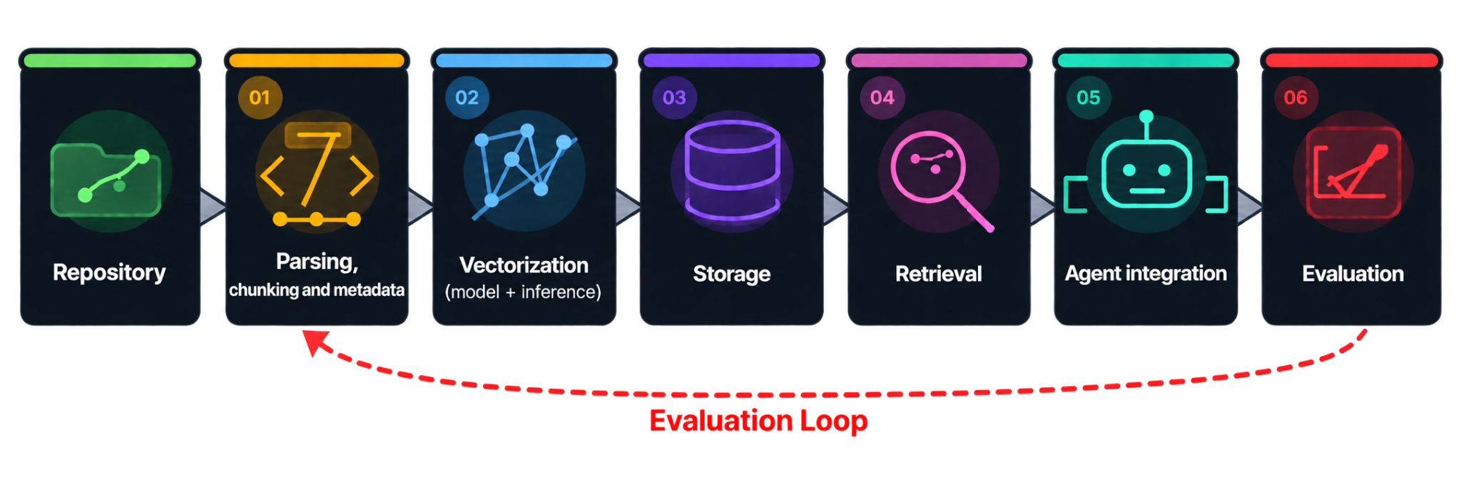
与 Agent 时代的许多好点子一样，其原生原型实现极其简单；但一个经过充分评估、达到生产级标准的解决方案，显然并非如此。在这一系列博客文章中，我们希望分享构建高效 RAG 系统所涉及的内容，以及我们在打造自有方案 Air Context 的过程中走过的弯路。我们将讨论从预处理、存储到 Agent 集成的每一个阶段，并提供更多技术背景和建议。

本系列第一部分将介绍管道的初始阶段：解析和分块，即将原始源文件划分为边界合理的单元；以及向量化，即将这些单元转换为支持语义搜索的表示形式。

解析与分块中的精细 AST

解析和分块是优秀 RAG 解决方案中的关键预处理步骤，但这一点经常被忽视。为了让 LLM 对源代码进行嵌入或以其他方式建立索引，我们首先必须向它提供原始代码行。这听起来或许微不足道，对于小型演示项目可能确实如此。然而，生产级系统包含数千个文件，而每个文件又可能长达数百甚至数千行。Agent 进一步加剧了这个问题，因为它们往往是高产的代码编写者，会继续扩大代码库。每个文件中都可能包含大量类、字段和方法，它们之间的关联程度各不相同。

找到合适的块大小

即使可以将这些庞大的代码文件完整放入嵌入模型中，这一昂贵操作最终也会适得其反。由于整个文件被嵌入为单个单元，搜索将返回整个文件。这与 Agent 式代码探索和导航的目标相悖，因为后者通常关注的是寻找特定函数、符号或代码片段。

另一方面，如果走向另一个极端，细粒度地嵌入每一行单独的代码，我们将面临另一类问题。脱离周边上下文时，这些单独的代码行在语义上可能并不重要。一个通用函数名或注释不值得单独嵌入，并且会产生错误的检索结果。某种意义上，我们会只见树木、不见森林，Agent 也会被大量通常并不重要的微小结果淹没。

因此，找到合适的方法来对代码进行分块或分组至关重要。每个组都应包含足够的必要上下文，并体现共同的语义含义。

为什么固定大小分块效果不佳

分块是对将要提供给 Agent 的内容进行划分、生成一组块的技术的统称。一种朴素的分块方法，是简单地将大文件切分为固定行数的多个组。然而，如果采用这种方法，我们会发现生成的分组在语义上并不正确。不相关的代码片段会被归在一起，例如 import 语句和某个函数的内容，从而导致检索错误。

为解决这一问题，我们可以利用这样一个事实：每个源文件都有相当明确的结构。以 Java 为例——import 通常位于文件顶部，接着是类定义，类头之前可能带有可选的文档注释。类中包含字段和方法，而这些内容也可能各自带有文档注释。了解定义类结构的惯例与规则，能让我们进行更智能的分块，并在周边信息上取得恰当平衡。

解析与结构感知分块

在过去 26 年中，JetBrains 开发了解析器，它们足够智能，能够适应特定语言中的各种特殊情况、不规则性、惯例和细微差别。这些解析器与其他工具一起，构成了我们的内部 JetBrains Code Engine 平台，Air Context 正是基于该平台开发的。截至本文撰写时，Air Context 支持对九种主要语言进行解析和结构感知分块：Kotlin、Java、Python、JavaScript、TypeScript、C#、PHP、Go 和 Rust。对于其他所有语言，我们的实现会直接回退到朴素的按行切分，以确保任何语言或文档都能被建立索引和搜索。

解析器使我们能够将源文件拆解为语法节点流，这些节点携带其所代表内容的信息——注释、空白、修饰符列表等等。随后，分块算法会消费该节点流，并应用用于决定某个块作用范围的逻辑。算法会基于节点类型、大小及其后代节点作出决策。如果一个节点超过大小阈值但没有子节点，算法将回退到更基础的切分策略。

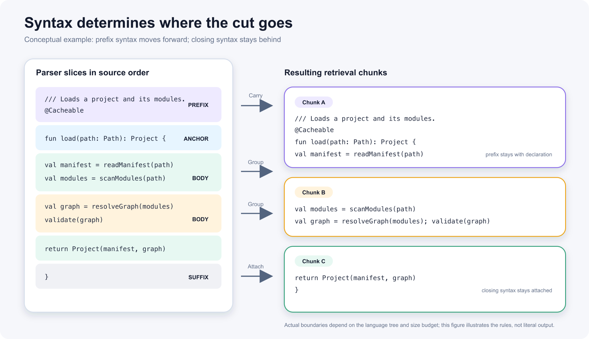
某些特定于语言的构造即使超过首选大小，也会保留为单个切片。文档、注解、可见性修饰符和关键字等前缀会与声明保留在一起；后缀（通常是闭合语法）则仍与其所闭合的构造关联。系统还会进行一些语言特定的清理，例如移除 Java 中常见但语义上没有意义的注解，如 @NotNull 或 @Override。

该算法与 Zhang 等人在 2025 年发表的 cAST 存在一些相似之处。我们的实现与 cAST 都会保留能够容纳的最大语法单元，只对过大的单元进行细分，并组合相邻的小单元，以避免生成通常不具备语义意义的微小块。最大的区别在于，我们在实现中编码了更多语言语义：例如，将 Python 装饰器与定义保留在一起，将 KDoc 与 Kotlin 声明放在一起，等等。

分组完成后，系统会执行块规范化，包括：

• 修剪开头和结尾的空白字符
• 删除空行
• 移除公共缩进，同时保留相对缩进

规范化完成后，该块会连同由相对路径构成的元数据一起传递到下一步——嵌入；相对路径会与规范化后的块内容一同被嵌入。

评估块的质量

很难对嵌入模型的输入应当是什么样子给出一个具体答案。块大小很重要，但如前文所述，更大并不总是更好。此外，与代码一起嵌入的某些元数据可能有用，而另一些则可能引入噪声，最终降低搜索质量。

我们选择使用 LLM-as-a-judge 策略，在评估中检查这些块。评审模型会使用一个块和对应源文件，判断其边界是否合理。它会寻找意外产物，例如脱离的文档、孤立的闭合语法，或从一个有意义的构造中间被截断的代码片段。此外，对源代码处理管道所做的任何改动，也都会通过完整的端到端检索评估。我们将在本系列下一部分回到这一评估管道。

向量化

在完成源代码预处理后，我们终于得到了大小合适、分组正确的文本块，以便进行语义检索。接下来的任务是通过称为向量化的过程，以一种能够在之后支持语义搜索的方式转换这些片段。

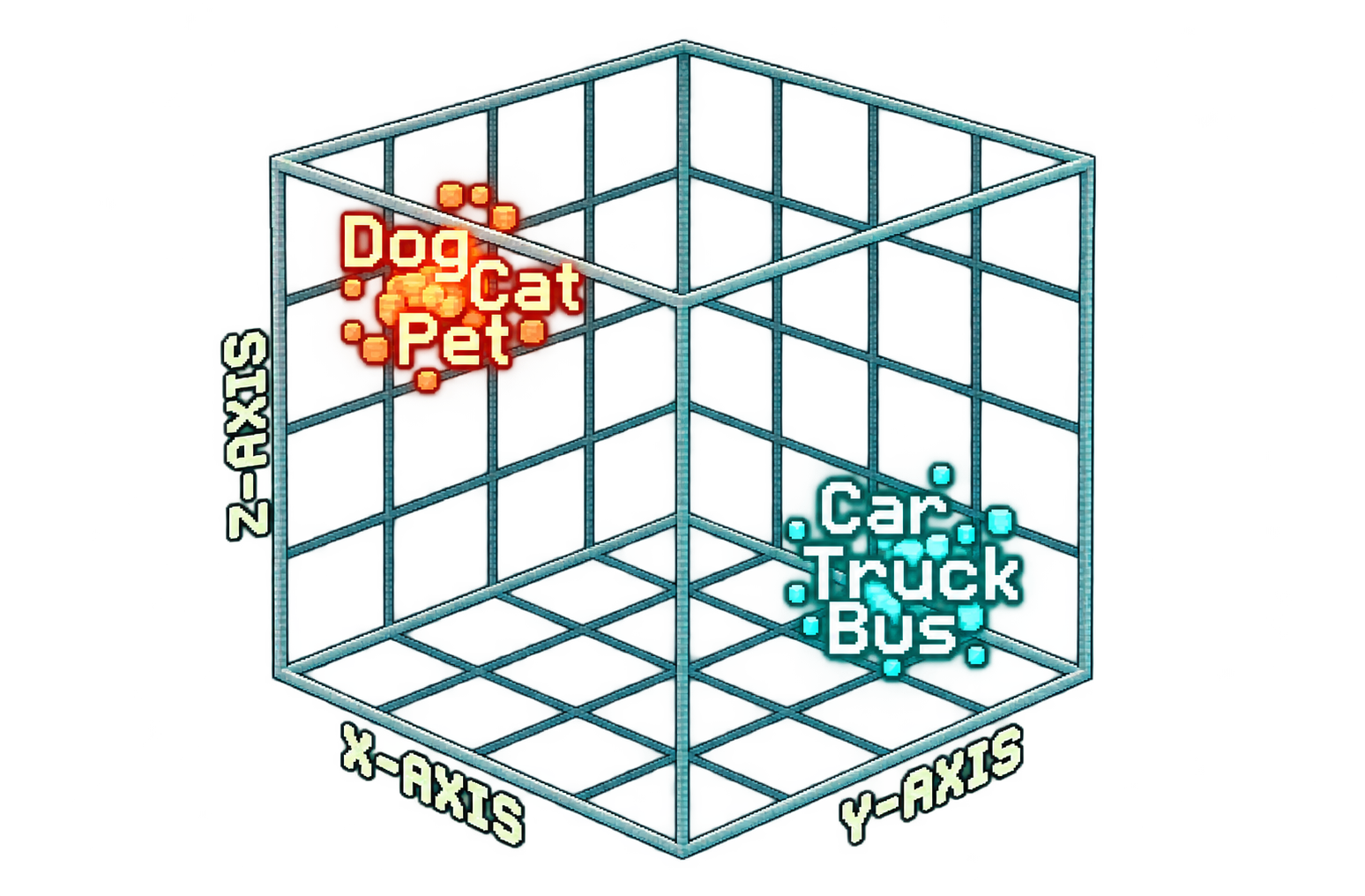
在向量化过程中，嵌入模型读取一段文本，并输出一个固定长度的数字列表（即向量）；这个向量相当于几千维空间中的一个点。重要的是，模型经过训练后，会让语义相近的文本落在彼此接近的位置。传统搜索可能无法发现它们之间的联系，但在这里，一个刷新缓冲写入操作的函数与一个清空待处理队列的函数，即使没有任何共同关键词，也可能彼此接近。因此，向量之间的距离成为相关性的衡量标准。查询会被转换为同一空间中的位置，距离它最近的内容就是结果。

每字节的性能：针对存储进行优化

任何将大型代码库向量化的尝试，都必须同时考虑成本和性能。单个嵌入很便宜，但大型仓库会产生数百万个块，继而变成数百万个向量；这些向量必须被存储、保留在内存中，并与每个传入查询进行比较。一个由 32 位浮点数组成、具有几千个维度的向量约占 16 千字节，因此在不考虑任何额外管理数据之前，几百万个块就会累积成数十 GB 的索引。在这一规模下，每个向量所分配的字节数成为成本限制因素，首要问题很快会从“我们能有多准确？”转变为“每字节能获得什么效果？”。换言之，我们需要在尽可能保留搜索质量的同时降低成本。

降低向量成本有两种方式。第一种是保留更少的维度。现代嵌入模型经过训练，使得向量开头的一段可以独立工作。维度损失会同时应用于多个嵌套的前缀长度，从而将最粗粒度的结构压入最早的维度。这意味着你可以截短一个向量并重新归一化，它仍然能够用于检索。另一种方式是保留每一个维度，但通过牺牲精度来减少每个维度的存储字节数。

这两个选项彼此独立，也可以组合使用，这意味着可以通过维度数量和数值精度的不同搭配来满足任何存储预算。真正的问题是：在相同字节数下，哪种搭配的检索效果最好？这种权衡远非均等。假设每个向量的预算是 512 字节。你可以将其用于保留 128 个维度，每个维度使用完整的 32 位精度；也可以保留全部 4,096 个维度，但每个维度只使用一个 bit。两种方案都恰好符合预算，但测试会发现，第二种方案的检索效果明显更好。

为什么维度比精度更重要

要理解其中原因，可以把每个维度看作模型学会向文本提出的一个小问题：这是否与错误处理有关？它是否涉及网络？这是否是测试代码？还有几千个类似的主题和问题尚未被命名。（真实的维度比这更模糊，但这是一个有用的抽象。）

单个答案本身并没有太大意义。当两个块针对许多此类问题给出相同答案时，我们便认为它们相似。因此，我们应通过问题的覆盖范围而非答案的精确程度来评估向量。

将全部 4,096 个维度保留为一位，能够为每个问题保留一个粗略的“是或否”答案。截断到 128 个维度，则只保留了百分之三问题的非常精确答案，并丢弃其余内容；而无论对保留下来的维度提高多少精度，都无法恢复被丢弃维度所承载的信息。从某种意义上说，一份填满勾选项的长问卷，胜过一份精确到小数点后六位的短问卷。维度是你希望保留的内容；精度则是你可以承受损失、并且更容易在后续补偿的内容。

因此，我们选择保留所有维度，并将精度降低推向极限，降

Agentic AI AI

Building a RAG Pipeline for Semantic Code Search: A Developer Diary and Field Notes

Part 1: Parsing, chunking, and vectorization

Some time ago, we set out to build the best semantic code search platform we could: a RAG pipeline that gives LLM agents precise, citable evidence from real repositories instead of whatever grep happens to surface. The eventual solution was Air Context. We got it working, we got it into production, and we collected a lot of scar tissue along the way. In this series of posts, we’ll share the parts we wish someone had told us on day one.

---

Coding agents are undoubtedly the biggest technology leap for software development of our decade. Agents and frontier models are proving their aptitude in the face of seemingly insurmountable code complexity to produce ostensibly reliable code.

However, as more and more development processes become agent-driven, the agent’s efficiency and the quality of the produced code become increasingly important. The question is not so much about whether an agent can complete the task, as given enough time and token resources, it surely will, but rather how much time, effort, and steering is required for it to generate production-grade results. For large-scale code bases specifically, the agent would spend a great deal of time searching for the relevant pieces of code relevant for the feature it’s working on and pulling them into the context.

Why semantic search matters

Attempting to locate the right code snippets, the agent will resort to traditional tools for code search such as keyword search and grep. These tools, however, are limited in that they require the agent to know in advance which exact text to search for. For example, an agent looking for where session tokens get refreshed cannot rely on the code helpfully containing the word “refresh”. To reason through abstract domains, the agent needs the ability to search for code by meaning, also known as semantic search. This is where retrieval-augmented generation (RAG) comes into the picture. If we can index the source code in a way that captures its semantics and then allow the agent to retrieve the relevant pieces on demand using free text search, we create an interface that plays to the agent’s strengths.

From prototype to production

Like many great ideas in the agentic era, a native, prototype implementation is extremely simple. A well-evaluated production grade solution most certainly is not. In this series of blog posts, we want to share what is involved in making an effective RAG system, as well as the wrong turns we took in our journey to create our own: Air Context. We’ll tackle each stage, from pre-processing to storage and agent integration, providing some more technical context and advice.

This first part of the series will cover the initial stages of the pipeline: parsing and chunking, where raw source files are divided into properly scoped units, and vectorization, where those units are transformed into a representation that supports semantic search.

The fine AST of parsing and chunking

Parsing and chunking is a critical pre-processing step in a good RAG solution, but it is often overlooked. In order to allow the LLM to embed or otherwise index the source code, we must first feed it the raw lines of code. This may sound trivial, and probably would be for small-scale demo projects. However, production-grade systems contain thousands of files, which, in turn, span hundreds or even thousands of lines. If anything, agents have compounded the problem, as they tend to be prolific writers, further inflating the codebase. Each file may contain multitudes of classes, fields, and methods, with varying degrees of relatedness among them.

Finding the right chunk size

Even if it were possible to fit these huge code files into an embedding model in their entirety, that expensive feat would ultimately be self-defeating. Because the entire file was embedded in a single unit, the search would return the entire file. This is counterproductive to the goals of agentic code exploration and navigation, which are mostly concerned with finding a specific function, symbol, or code snippet.

On the other hand, if we were to take the other extreme and granularly embed each separate line of code, we would be facing a problem of a different sort. These individual lines can be semantically insignificant without the surrounding context. A generic function name or comment does not merit embedding and will produce the wrong retrieval result. In a sense, we would not be able to see the forest for the trees, and the agent would be overloaded with multiple, often insignificant micro-results.

It is therefore imperative to find the right method to chunk or divide the code into groups that are properly scoped. Each group should include enough of the necessary context and represent common semantic meaning.

Why fixed-size chunking falls short

Chunking is a generic name for the technique of taking content that will be fed to the agent and dividing it into a set of chunks. A naive approach to chunking could be simply splitting a large file into groups with a fixed number of lines. However, if we were to take that approach, we would find the resulting groupings semantically wrong. Unrelated code pieces would be grouped together, for example, an import statement and some function content, leading to mistakes during retrieval.

To solve the problem, we can leverage the fact that every source file has a pretty well-defined structure. Take Java as an example – imports tend to be at the top of the file, followed by a class definition with an optional doc-comment preceding the header. The class will contain fields and methods, which in turn may also have their own doc-comments. Knowing about the conventions and rules that define the class structure allows us to perform smarter chunking and achieve the right balance of surrounding information.

Parsing and structure-aware chunking

Over the last 26 years, we at JetBrains have developed parsers that are smart enough to adjust for the various quirks, irregularities, conventions, and nuances of specific languages. Alongside other tools, these parsers form our internal JetBrains Code Engine platform on which Air Context is developed. At the moment of this article’s composition, Air Context supports parsing and structure-aware chunking for nine major languages: Kotlin, Java, Python, JavaScript, TypeScript, C#, PHP, Go, and Rust. For all other languages, our implementation simply falls back to naive, line-based splitting to ensure that any language or document can be indexed and searched.

The parser allows us to break source files into streams of syntax nodes that carry information about what they represent – comments, whitespaces, lists of modifiers, and so on. The chunking algorithm then consumes that stream and applies logic that decides the scope of a given chunk. Based on the node’s type and size, as well as its descendants, the algorithm makes a decision. If a node exceeds the size threshold but has no children, it will fall back to more primitive splitting strategies.

Some language-specific constructs are kept as single slices even if they exceed the preferred size. Prefixes such as documentation, annotations, visibility modifiers, and keywords are kept together with the declaration; suffixes (usually closing syntax) remain associated with the construct they close. There is also some language-specific cleaning, where, for instance, common and semantically meaningless Java annotations such as @NotNull or @Override are removed.

The algorithm bears some similarities to cAST, authored by Zhang et al. in 2025. Both our implementation and cAST retain the largest syntax units that fit, subdividing only the units that are too large, and grouping smaller adjacent units to avoid tiny chunks that are not usually semantically meaningful. The biggest difference is that we coded more language semantics into our implementation, keeping Python decorators together with definitions, KDocs next to Kotlin declarations, and so on.

After grouping, chunk normalization is performed, which involves:

• Trimming leading and trailing whitespaces
• Deleting blank lines
• Removing common indentation while preserving relative indentation

Following the normalization procedure, the chunk is then passed to the next step – embedding – along with metadata that consists of a relative path, which gets embedded alongside the normalized chunk content.

Evaluating the quality of chunks

It is hard to give a concrete answer as to what the input to the embedding model should look like. Chunk size matters, but as discussed before, bigger is not always better. Additionally, some metadata embedded alongside the code may be useful, while some may introduce noise that ultimately decreases search quality.

We opted to use an LLM-as-a-judge strategy to inspect the chunks as a part of the evaluation. The judge, using a chunk and the source file, considers whether the boundary makes sense. It looks for unexpected artifacts, such as detached documentation, orphaned closing syntax, or fragments of code that are cut through a meaningful construct. In addition, any changes to the source code processing pipelines also go through the full, end-to-end retrieval evaluation. We’ll get back to that evaluation pipeline in the following part of this series.

Vectorization

Having pre-processed the source code, we finally have text chunks that are hopefully just the right size and correctly grouped for semantic retrieval. Our next task is to transform these fragments in a way that will later allow us to support semantic search, through a process called vectorization.

With vectorization, an embedding model reads a piece of text and emits a fixed-length list of numbers (a vector), which amounts to a point in a space of a few thousand dimensions. Significantly, the model is trained so that texts with similar meaning land close together. Traditional search might miss the connection, but here, a function that flushes buffered write operations and one that drains a pending queue can end up near each other despite sharing no common keywords. The distance between vectors hence becomes a measure of relatedness. A query is turned into a position in the same space, and the results are whatever lies nearest to it.

Punch for the byte: Optimizing for storage

Any attempt to vectorize a large codebase must take into account both cost and performance. A single embedding is cheap, but a large repository produces millions of chunks, which become millions of vectors that must be stored, held in memory, and compared against each incoming query. A vector of a few thousand dimensions in 32-bit floats weighs around 16 kilobytes, so a few million chunks add up to tens of gigabytes of index before any bookkeeping. At such a scale, the allocation of bytes per vector becomes cost-limited, and the leading question quickly shifts from “how accurate can we be?” to “what do we get per byte?” In other words, we need to find a way to reduce the cost while retaining as much search quality as possible.

There are two ways to reduce vector cost. The first is to keep fewer dimensions. Modern embedding models are trained so that a leading slice of the vector works on its own. The dimension loss is applied across several nested prefix lengths simultaneously, pushing the coarsest structure into the earliest dimensions. This means you can cut a vector short and renormalize it, and it still retrieves. Alternatively, you can keep every dimension and spend less on each one by sacrificing on precision and thus keeping fewer bytes for each vector.

These two options are independent of each other and can be combined, which means any storage budget can be met through different mixes of dimension count and numeric precision. The real question is which mix retrieves best for the same number of bytes. The trade-off is far from even. Suppose the budget is 512 bytes per vector. You could spend it on 128 dimensions kept at full 32-bit precision, or on all 4,096 dimensions kept at a single bit each. Both fit the budget exactly, but in testing, you’ll find that the second option retrieves considerably better.

Why dimensions matter more than precision

To see why, it helps to think of each dimension as one small question the model has learned to ask about the text: Is this about error handling? Does it touch the network? Is it test code? And there are a few thousand similar topics and questions that haven’t been named. (The real dimensions are blurrier than that, but this is a useful abstraction.)

No single answer means much on its own. We consider two chunks to be similar when their answers to many of these questions are the same. Therefore, we should assess the vectors by looking at the coverage of the questions rather than the exactness of the answers.

Keeping all 4,096 dimensions at one bit preserves a rough yes-or-no answer to every question. Truncating to 128 dimensions keeps very precise answers to three percent of the questions and throws the rest away, and no amount of precision on the surviving dimensions can recover the information the discarded ones carried. In a sense, a long questionnaire filled in with checkmarks beats a short one filled in to six decimal places. Dimensions are what you want to keep; precision is what you can afford to lose and is easier to compensate for later on.

So we chose to keep every dimension and take the precision reduction to its limit, dropping the vectors to one bit each, which is 32 times smaller than the same vector in 32-bit floats. The quantization itself turns out to be surprisingly simple. Every component at or above zero becomes a one, while every negative component becomes a zero, and the magnitudes are thrown away:

Changing the representation changes the metric with it. Cosine similarity needs the magnitudes we just threw away, so binary vectors are compared by Hamming distance instead, which is simply the number of positions where two bit patterns disagree. Compare, for example, 10110100 and 10010110. They differ in two positions, so the distance between them is two. At full length, the computation stays just as simple. A 4,096-bit vector is stored as 64 words of 64 bits, and comparing two of them means XORing each pair of words, which leaves a 1 wherever the two vectors disagree, and then counting the 1s. A CPU does each of those in a single instruction per word, so a full comparison costs in the order of a hundred instructions where cosine similarity on the original floats needed thousands of multiplications.

Note that the metric was never a separate decision. We chose one-bit precision for the storage savings, and once every component is a sign bit, Hamming is the only comparison left that makes sense. Choosing the precision chose the metric.

Binary quantization still costs a few points of recall against the unquantized vector. We accepted that cost after considering that a reasoning agent would be consuming the results. A code search feeding an agent needs the right neighborhood far more than a perfectly ordered top 10. When the agent asks where session tokens get refreshed, what matters is that the relevant handful of files shows up among the first dozen results. Whether the best chunk ranks second or fifth changes nothing, because the agent opens the candidates and reads them anyway. In that loop, a ranking degradation that would be plainly visible in a three-result UI built for humans is mostly invisible.

The limits of binary quantization

The trade-off we made had a subtler cost that took us a bit longer to understand. Binary quantization doesn’t only sacrifice accuracy; it compresses the range of similarity scores. With full-precision vectors, an unrelated pair can score near zero while near-duplicates score near one, a comfortably wide spread. Sign bits behave differently. Around half the bits of two entirely unrelated vectors still agree by pure chance, while a strongly related pair might have agreement for two-thirds. So every score in the index, relevant or not, lands in that thin band.

Ranking survives the compression, since relevant results still score above irrelevant ones, but thresholding does not. Picture a feature that volunteers related code without being asked, say a panel that suggests existing implementations while you type. Its most difficult requirement is knowing when to stay silent. To make that determination, it needs a usable gap between “related” and “unrelated” scores. Binary vectors don’t leave one. Any cutoff placed inside that narrow band either fires on everything or on nothing. So where an index needs an absolute relevance judgement rather than a relative ordering, we keep 16-bit floats and pay for the storage.

Embedding scope

While indexing and searching use the same model, the two jobs could not be more different. Indexing is throughput-constrained, with millions of chunks asynchronously handled. The GPU will handle about 32 chunks per batch before becoming saturated. A search, on the other hand, needs to be fast and responsive. Users will give up if they are not provided with results within a couple of seconds at most. Therefore in deploying these models we optimize them accordingly: one to maximize chunks per second, the other for minimizing time to first result.

We chose an instruction-following model, trained with a deliberate asymmetry between the two sides of retrieval. Significantly, the two sides are represented by very different types of text. A query is a short question in natural language, while a document is a chunk of code. A document is embedded as is at indexing time. A query is wrapped with an instruction describing the retrieval task, something like “given this search query, find the code that answers it”, which tells the model what role the text is playing. We preserve that arrangement at inference because it is the shape the model learned.

To allow the two sides to align more easily, we embed each chunk together with its file path. The path supplies metadata that the chunk alone lacks: which module it lives in, and what the file is. In a monorepo, though, the path itself becomes a problem. The IntelliJ IDEA monorepo runs to over a million files. The median source file there sits nine directories deep behind a 91-character path, and close to 10,000 source files have paths longer than 150 characters, the longest of them 218. That is before any checkout root is prepended.

Most of those characters are used for structural nesting and offer no useful information about the file. A run of segments like src/org/jetbrains/kotlin/idea/k2 restates the package hierarchy, which a compiler needs and a search does not. Meanwhile, the file at the end of that longest path is 24 lines long. If we simply embed the path text as is beside a chunk, we’ll find that the path will sometimes take up more space than the code itself. To compensate for that, a path is capped before it reaches the model, and the rule is that both ends survive. The leading segments tell you which module you’re in, while the last two, the immediate parent and the filename, tell you what the file is. The middle is the part that can go, and only as much of it as the cap requires. Keep the longest prefix that still fits, elide what falls between into …, and if even parent-plus-filename is too long, keep only the name itself.

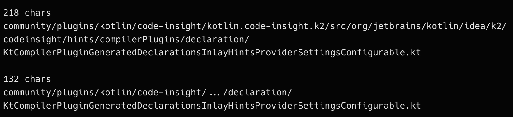
The same discipline applies when a user scopes a search to a subdirectory. The obvious implementation is a metadata filter: run the search as usual and discard results that fall outside the directory. We do something different. The scope is rendered into the query text itself, in the same shape, with the same abbreviation function and the same separator the indexed chunks used. If a chunk went into the index under the abbreviated form of community/plugins/kotlin, a query scoped to that directory carries the same string in exactly the same form, so the query vector lands in the same region as the chunks it is supposed to match.

Protecting source code

There was one last design consideration we took into account. It was important for us to be attentive to customer privacy and security concerns. The source code of a company is often the core of its IP. Exposing it to third-party cloud models, or even to another company, increases the risk of inadvertently exposing sensitive data or even training other models to use it.

To make sure we address these concerns, we made the decision to adhere to several practices early on:

1. Avoid storing the code in our systems: A chunk holds a cluster reference, an item type, a file path, start and end offsets, a reference to a vector, and an optional metadata field. No content, no copy of the source code itself, is saved. What a search returns is coordinates, and the snippet you see is assembled on your machine, from your checkout, using them. The server just knows that something relevant lives at bytes 4,102–4,890 of a given path, not what it is.
2. Don’t use data for training: Every code index Air Context builds is embedded by an open-weight embedding model, running on GPUs we operate. No embedding request leaves our infrastructure – not to OpenAI, not to Google, not to any other vendor. Therefore, we can guarantee that none of the data will be used to train anything.

These self-imposed design restrictions carry no cost in terms of retrieval quality. We evaluated the open-weight candidates against the hosted embedding APIs from the major providers on our own code-retrieval benchmarks, and ours came out on top. Open-weight embedders are now good enough that the interesting engineering has moved into what you feed them, how you serve them, and what you choose to keep.

A summary that is an interlude

In this blog post, we covered the first stages of the retrieval pipeline: the journey from raw source files to compact vectors that are ready to be searched.

At this point, we have millions of binary vectors and a way to produce more. The problems we haven’t solved yet are how to store them efficiently, how to create a system that can answer a query in milliseconds, how we can continuously evaluate our results to ensure we are making the right choices, and how we can get the agent to actually use our shiny RAG apparatus.

These topics and more will be the subjects of the next parts in this series, which we’ll be releasing over the next few weeks. As always, please feel free to ask any questions in the comments or share your own hard lessons from designing a RAG solution. We are eager to learn of different and creative ways you have found to be effective! In the meantime, feel free to check out Air Context, currently in public preview, it is already included with your JetBrains license 😀

Until next time!

Subscribe to JetBrains AI Blog updates